Error Diffusion Dithering

What error diffusion dithering is

Error diffusion is a digital halftoning technique that reproduces a continuous-tone (multi-level) image on an output device or file format supporting only a limited number of levels — in the extreme case, a two-level (bi-level) device — by quantizing each pixel to the nearest available level and then distributing the resulting quantization error to neighboring pixels that have not yet been processed. Reference sources define it precisely as a type of halftoning in which the quantization residual is distributed to neighboring, not-yet-processed pixels.

The defining idea is a feedback loop that conserves error locally. Ordinary thresholding rounds each pixel to the nearest level and discards the difference; error diffusion instead carries that difference forward, so that across a small neighborhood the average intensity of the output closely tracks the average intensity of the input. This local averaging is what allows a device with only a few ink, toner, or display states to convey the appearance of many intermediate tones.

Error diffusion belongs to the broader family of halftoning and dithering methods surveyed in the companion Halftoning overview, which covers amplitude-modulated (AM) versus frequency-modulated (FM) screening, screen ruling, screen angles, and dot gain at a high level. This page does not restate that material; instead it goes deeper on the error-diffusion family specifically — its mechanism, its diffusion kernels, the effect of scan order, its characteristic artifacts, and how it relates to ordered dithering and thresholding. In the halftoning taxonomy, error diffusion is one of the FM (stochastic) approaches, producing dispersed, aperiodic dot patterns rather than a regular periodic screen.

How the algorithm works

Error diffusion processes pixels in a defined order — conventionally left to right, top to bottom — and performs two operations at each pixel: quantization, then error distribution. Expressed as a single pass, the steps are:

• Read the current pixel value, including any error already propagated to it from previously processed neighbors.
• Quantize it to the nearest available output value. For a bi-level target this is a single threshold (rounding) decision; for a limited palette it is the closest palette entry.
• Compute the quantization error as the difference between the value used in the calculation and the quantized output actually emitted.
• Distribute that error to a fixed set of not-yet-processed neighboring pixels, scaled by the weights of a diffusion kernel, adding the weighted fractions to those neighbors before they are quantized in their turn.

Because the weights of a kernel normally sum to one (the whole error), the total error is conserved and pushed ahead of the moving quantization front; some kernels deliberately propagate less than the full error, a design choice discussed below. A pixel is only ever adjusted by errors arriving from neighbors that were already visited, which is why the method completes in a single pass and never revisits a pixel.

The per-pixel quantization at the heart of the loop is itself a thresholding operation — the same nearest-level decision described in the Image Thresholding reference. What distinguishes error diffusion is the feedback path that plain thresholding lacks: the residual is not thrown away but transported to nearby pixels. A consequence is that each output value depends on the accumulated decisions of all previously processed pixels, making the computation recursive and order-dependent rather than a set of independent per-pixel choices.

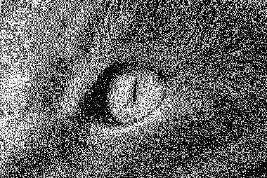
The Floyd–Steinberg kernel and its origin

The most widely cited error-diffusion algorithm was published by Robert W. Floyd and Louis Steinberg in 1976, in a paper titled "An Adaptive Algorithm for Spatial Gray Scale" in the Proceedings of the Society for Information Display (volume 17, pages 75–77). A closely related "minimized average error" method was disclosed nearly concurrently by J. F. Jarvis, C. N. Judice, and W. H. Ninke at Bell Labs, so error diffusion is best understood as emerging from parallel work in the mid-1970s rather than from a single definitive origin.

Floyd–Steinberg distributes the quantization error of the current pixel to four not-yet-processed neighbors, using a divisor of 16. The pixel immediately to the right of the current pixel receives 7/16 of the error; on the next row down, the pixel below-left receives 3/16, the pixel directly below receives 5/16, and the pixel below-right receives 1/16. These four fractions sum to 16/16, so the entire error is propagated forward.

The weights are largest for the pixels nearest the current one and are biased toward the forward scan direction and the following row, spreading the error locally while keeping the kernel small. Its compactness — only four neighbors — makes it inexpensive to compute, which contributed to its wide adoption; the larger kernels described next spread error more smoothly across more pixels at greater computational cost.

Diffusion kernels and named variants

Many error-diffusion kernels have been published, differing in how many neighbors they touch and in their weights and divisor. Larger kernels distribute the error over more pixels and more rows, which tends to smooth the result and suppress some artifacts, at the cost of more computation and greater spatial spreading of each error. Widely catalogued examples include:

• Jarvis, Judice, and Ninke (JJN): a Bell Labs "minimized average error" kernel disclosed nearly concurrently with Floyd–Steinberg; it spreads error across the current row and the next two rows, with a divisor of 48.
• Stucki: an adjustment of the JJN kernel using a divisor of 42, presented as a refinement aimed at processing efficiency.
• Burkes: a two-row kernel derived from Stucki (dropping its bottom row) that returns to a power-of-two divisor of 32.
• Sierra family: the three-row Sierra kernel (divisor 32), the smaller Two-Row Sierra (divisor 16), and the compact Sierra Lite (divisor 4), trading breadth of diffusion for speed.
• Atkinson: devised by Bill Atkinson and used on early Apple Macintosh computers; it adds one-eighth of the error to each of six neighbors and therefore propagates only three-quarters of the total error. Deliberately discarding part of the error raises local contrast and reduces speckle, but can clip detail in the deepest shadows and brightest highlights.
• Ostromoukhov's variable error diffusion: introduced by Victor Ostromoukhov, it varies the diffusion coefficients according to input intensity and uses a serpentine scan, producing output with a blue-noise character intended to suppress the structured artifacts of fixed kernels.

There is no single "correct" kernel. The choice trades computational cost, sharpness, smoothness, and the type of residual artifact, and the appropriate kernel depends on the output device, its resolution, and the image content.

Scan order: raster, serpentine, and 1D versus 2D

Because error is only ever pushed toward pixels that have not yet been processed, the order in which pixels are visited affects the result. A plain raster order — every line scanned left to right — propagates error consistently in one horizontal direction, which can imprint a directional bias on the output.

Serpentine scanning, also called boustrophedon, alternates the horizontal scan direction on each successive line: left to right on one line, right to left on the next. Reversing the direction line by line breaks up the consistent directional transport of error and commonly reduces uniform speckle and some directional patterning, at the cost of a slightly more complex implementation.

The dimensionality of the kernel matters as well. One-dimensional error diffusion, which pushes error only along the current line, tends to produce pronounced artifacts that show up as distinct vertical lines. Two-dimensional kernels, which also push error into the next row, distribute it more evenly and reduce these visual artifacts — one reason practical implementations use two-dimensional kernels such as those listed above.

Characteristic artifacts and refinements

Error diffusion generally renders fine detail and smooth gradients well, but its feedback structure can introduce characteristic artifacts, most visible in large flat areas and near the extremes of the tone range. Because each output depends on the running accumulation of earlier errors, correlated and structured textures can appear — sometimes described in the literature as directional streaks or "worm"-like patterns — particularly with fixed kernels and plain raster scanning.

Near solid highlights and shadows, the slow accumulation of small residual errors can leave sparse isolated dots or short transient patterns before the output settles. Partial-error kernels such as Atkinson's mitigate this by not carrying the full error forward, at the expense of clipping the most extreme tones.

Several strategies reduce these artifacts:

• Serpentine (boustrophedon) scanning, to break the consistent directional bias of plain raster order.
• Larger, two-dimensional kernels (such as Jarvis–Judice–Ninke or Stucki) that spread each error over more neighbors.
• Variable-coefficient methods, such as Ostromoukhov's, which adapt the weights to tone and aim for a blue-noise spectrum.

Blue noise refers to a spatial distribution dominated by high-frequency (fine-grained) structure with little low-frequency clumping; the human visual system tolerates it well, which is why it is a common target for good stochastic patterns. Error diffusion is one way to approximate a blue-noise distribution on a limited-level device.

Relationship to thresholding and ordered dithering

At its core, error diffusion makes the same per-pixel decision as thresholding: mapping a continuous value to the nearest available output level. The difference is the feedback loop. Plain thresholding discards the rounding error at each pixel, so it cannot represent intermediate tones and produces hard, posterized boundaries; error diffusion conserves that error by spreading it to neighbors, recovering apparent tone through spatial averaging. The Image Thresholding reference covers the quantization and binarization decision itself in more depth.

Ordered dithering pursues the same goal by a different route. It compares each pixel against a position-dependent threshold read from a small, fixed matrix — for example a Bayer matrix — tiled across the image. Because each pixel's decision depends only on its own value and its location within the matrix, and not on any other pixel's output, ordered dithering is a point operation: it is fully parallelizable and produces a regular, periodic pattern.

Error diffusion, by contrast, is recursive. Each output depends on the outputs of previously processed pixels, so the computation is inherently sequential along the scan and harder to parallelize. In exchange, its patterns are aperiodic and adapt to image content, which typically renders fine detail and gradients with fewer periodic textures than a fixed ordered matrix. Neither approach is universally superior: ordered dithering is faster and trivially parallel, while error diffusion generally offers better tonal detail but is more computationally involved and can exhibit the directional artifacts described above.

Relationship to halftoning, FM screening, and the print pipeline

Error diffusion is itself a form of digital halftoning — it is defined as a halftoning method in which the quantization residual is distributed to neighboring pixels. Within the taxonomy set out in the Halftoning overview, it belongs to the frequency-modulation (FM), or stochastic, family: it varies the placement and number of small, similar marks rather than the size of dots on a fixed grid, yielding an aperiodic pattern with no dominant screen frequency or angle.

Having no regular grid, error-diffusion output largely avoids the moire that can arise when periodic AM screens overlap or interact with regular image detail, and it can resolve very fine detail. The same absence of a coarse, robust dot structure makes FM-type output — including error diffusion — more sensitive to dot gain and press variation in physical printing; the Halftoning reference discusses those substrate and press considerations for FM/stochastic screening in general, and they are not repeated here.

In a print workflow, screening of this kind is applied at raster/output time by a Raster Image Processor (RIP) or by printer firmware, after the page has been rasterized to the device's addressable grid and before the resulting bi-level bitmap drives the marking engine. Many desktop and office laser and inkjet printers rely on error-diffusion-style FM screening for photographic and grayscale output; see the Raster Image Processor reference for where screening sits in the overall pipeline.

Practical use, advantages, and limitations

Error diffusion is used wherever a limited-level device or format must approximate continuous tone. Common applications include:

• Bi-level and few-level printing — laser and inkjet engines that place essentially on/off marks, where error diffusion supplies an FM-type screen. Applied to each process color, it extends to color printing (see the CMYK reference).
• Color quantization to a limited palette — reducing a full-color image to an indexed palette, such as low-color-count image formats, while preserving apparent tonal range.
• Low-bit-depth displays — presenting many apparent tones on panels or displays that support only a few levels per channel.

Its principal advantages are:

• Strong reproduction of fine detail and smooth gradients for a given output resolution.
• Aperiodic, content-adaptive output that avoids the periodic patterning and moire associated with fixed screens.
• Good implementations approximate a blue-noise spatial distribution, which the eye tolerates well.
• Conservation of local average intensity, so overall tone is preserved even on a strictly bi-level device.

Its principal limitations are:

• It is inherently sequential — each output depends on earlier ones — so it is harder to parallelize than point-wise ordered dithering.
• It can produce directional or correlated textures (streaks or "worm"-like patterns) in flat regions, mitigated but not always eliminated by serpentine scanning and variable-coefficient kernels.
• Fixed kernels can leave sparse-dot or transient artifacts near tonal extremes; partial-error kernels reduce these but clip extreme highlights and shadows.
• As an FM-type screen, physical prints are more sensitive to dot gain and press variation than coarse AM screens.
• Results depend on kernel choice, scan order, and image content, and no single configuration is optimal for every case.

This is a neutral technical reference; figures, kernel weights, and the attribution above are drawn from the documented sources listed below and do not include pricing, marketing claims, or product recommendations.